A mini guide to Eigenfunctions
If you are following my article series on Quantum computing you may have come across the term eigenfunction or eigenstate. I started to try to outline the meaning of these concepts in place, but the blogs quickly got a bit bogged down in the side note so I have pulled the topic out into its own piece. I hope you will digest and enjoy the introduction below and then return to one of my fuller articles.

Remember eigenvectors?
Hopefully I’m starting with something you know about, eigenvectors. Recall that an eigenvector v, and eigenvalue λ, of a matrix M, is a vector such that:
M(v) = λ(v)
In other words, the transformation M leaves the vector v scaled by the scaler eigenvalue λ, but its direction unchanged. Any matrix can have one or more eigenvectors and each eigenvector will have a corresponding eigenvalue.
In quantum mechanics this concept is expanded to more complex linear transformations on abstract vector spaces that represent quantum properties. We learnt earlier that you can represent quantum systems using a Hilbert space. Vectors in Hilbert spaces are wave functions so in quantum computing we work with eigenfunctions instead of eigenvectors. A transformation T with eigenfunctions f and eigenvalue λ would look like this, where f is an eigenfunction of T because applying T scales f linearly, but otherwise leaves it unchanged. It probably worth remembering that λ can be a complex scalar.
T f(x) = λ f(x)
It is always easier to understand these things with an example. Lets let transformation T be the differential operator. The differential operator is a function that takes a function and returns another. We are used to applying the differential operator, but we don’t usually frame it in those terms. For the differential operator the function eˣ is an eigenfunction because after applying differentiation the function is simply scaled. I chose this example deliberately as we will come back to differential operators later when we look at quantum operators in related posts.

The Schrödinger equation in its simplest form is an eigenequation:

In this equation |𝛹⟩ is the wave function which describes the quantum state of the system. H-hat is the Hamiltonian, a quantum operator that describes the energy of the particles of the system and their interactions. E is the total energy of the system.
Here the wave function |𝛹⟩ is an eigenfunction of the Hamiltonian operator meaning that any application of the Hamiltonian to the wave function will result in the same function |𝛹⟩, but scaled by E, the eigenvalue. A solution to the Schrödinger equation for any given Hamiltonian H, is a wave function that satisfies this property.
In quantum mechanics eigenfunctions are also often called eigenstates. They are not quite the same, but for the moment we can use the terms interchangeably. Any eigenfunction or eigenstate in a quantum system in respect of an observable property is a state in which that observable has a specific value. If a system is in a an eigenstate with respect to some observable then measuring the system will yeild the eigenvalue of that eigenstate. In that respect quantum operators are somewhat analogous to performing a measurement of the system: on a physical system we can determine an eigenvalue of the eigenstate by measuring the observable, on paper if we have a quantum operator and a wave function we can apply that operator to that wave function to find the eigenvalue.
If a quantum system is in a superposition of eigenstates then measuring the system will result in the eigenvalue of one of the eigenstates. The wave function gives us the probability that the measurement with yield that eigenvalue. When talking about quantum systems we often drop the eigen- and everything feels much less like hard work.
In quantum computing, we talk about qubits having two base states: |0⟩ and |1⟩. These are eigenstates that have eigenvalues that correspond to measurements we have assigned to meaning 0 and 1. For example spin up and spin down. If we were to construct the Schrödinger equation for a qubit, the states represented by |0⟩ and |1⟩ would be solutions. The eigenvalues of those eigenstates are what is actually measured.
I talk about what constitutes quantum measurement in more detail in previous articles. That is a rabbit hole that requires a lot more thought.