Quantum Prime Factorisation: Shor’s algorithm
Shor’s algorithm is a big deal because it is a method of quickly finding the prime factors of a very large number. This is very hard to do with a classical computer and is used in almost all modern encryption. Encryption is what protects our banking systems, medical data and selfies from falling into the wrong hands.
Breaking down the factoring problem into a different problem
Through some really fun numerical algebra we can break down the problem of factorising a large number N into a different problem, which we can solve with a quantum computer.
Shor’s algorithm is as follow:
Shor’s algorithm works for prime factorisation in general, but for simplicity lets consider that given a large number N, we want to find prime numbers p and q such that N = pq.
1. Pick a random number x < N
2. Find k = gcd(a,N), the greatest common divisor of a and N, easily calculated with Euclid’s algorithm
3. Assuming k > 1 then k = p and we are done. Otherwise use a quantum computer to find the order r of x and N such that xʳ mode N = 1
4. If r is odd then try again with a new random x, otherwise we find g = gcd (N , xʳᐟ² -1). If g > 1 then we are done and g = p. If g = 1 then our random number was bad and we restart with a different x.
How does this work?
Step 2 relies on the ease of finding the greatest common divisor using Euclid:
if g = gcd(A, B)
⇒ A = αg and B = βg for some α,β because by definition g divides A and B.
⇒ A-B = αg-βg = (α-β)g
⇒ g = gcd(B, A-B) = gcd (A’, B’)
You can then repeat until A’ = B’
Step 3 relies on some number theory which says that the numbers less than N and coprime to N form a group and that for any x in that group there exists a multiplicative order r that satisfies xʳ mode N = 1, where r is the smallest number for which that holds.
Step 3 also relies on the idea that we can find r easily with a quantum computer. Finding r with a classical computer is harder than finding the factors of N by brute force so it is a pointless transformation of the algorithm unless you have a quantum computer handy.
Step 4 is a bit more tricky. If r is even then we can write the following
xʳ mode N = 1
⇒ N | xʳ — 1 which mean N divides xʳ — 1
⇒ N | (xʳᐟ²-1)(xʳᐟ² + 1) We can factor like this because r is even.
We know that N cannot divide (xʳᐟ²–1) because r is the smallest number such that N divides xʳ — 1, but it is possible that N divides xʳᐟ² +1. We compute g = gcd (N , xʳᐟ² -1). If g = 1 then that means that xʳᐟ² -1 is coprime to N, which means that N divides xʳᐟ² + 1 and we need to restart with a different guess x.
Before we look at the quantum part, lets convince ourselves that this works:
I’m going to choose to factor 77:
Let x = 10
r = 6 // using a spreadsheet to brute force
g = gcd (77, 10³–1) = 1 // oh dear, start again
Let x = 12
r = 6
g = gcd (77, 12³–1) = 11
We are done 77 = 7 x 11
Using some further number theory you can show that x is going to be a good guess at least half the time so the algorithm works quickly. We’ll come back to that later.
So how do we find r with a quantum computer?
We find r using a quantum subroutine called Quantum Phase Estimation (QPE).
Remember that we want to find r such that r is the smallest number that satisfies the following for N and our guess x.
xʳ mod N = 1
With a classical computer we can try different values of r until we get the right answer. With a quantum computer we can try all values of r and all values of xʳ mod N at the same time using superposition to represent all values of r simultaneously. The trick is then manipulating the qubits so that we only get the right answer when we measure them.
The Quantum Algorithm
We start with a quantum computer with two registers, A and B, before applying a series of gates and then measuring the value of register A. How big are those registers? Register B will have n qubits such that N ≤ 2ⁿ. Early estimates for Register A suggested m qubits where N² ≤ 2ᵐ < 2N², but it has subsequently been shown that 2n qubits is sufficient to find r.
The numbers x (our guess to start the algorithm) and N (the number we are trying to factorise) are not going to change so their values are built into the design of the quantum circuits and we don’t need to hold them in a quantum register.
Next we put the register A into a superposition representing all numbers a < 2²ⁿ. This is easy since we can just put every bit in register A in a superposition that is equally likely to be measured as |0⟩ or |1⟩. This means that the register as a whole contains a superposition of all numbers 0 to 2²ⁿ with equal probability of any number being measured. You can do this by transforming each qubits in to the state (|0⟩ + |1⟩)/√2 using the Haramard gate:
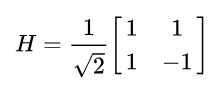
The Haramard gate is one way of transforming a qubit with known state of |0⟩ or |1⟩ into a qubit with superposition that has equal probability of |0⟩ or |1⟩. If we started with each qubit in state |1⟩ then we would end up with (|0⟩ - |1⟩)/√2 instead. The matrix above is just another way of expressing this transformation on states |0⟩ and |1⟩.
Next we calculate xᵃ mod N = k in register B. This can be done in a way similar to the way we do it in classical computing. You first raise x by all powers of 2 then you multiply those powers of 2 if there is a corresponding 1 in the binary representation of a. The register A holds all values of a < 2²ⁿ, so register B holds all values of xᵃ mod N = k.
power(int x, bool[] a, int m, int N) {
int k = 1;
  for (i = 0, i < m, i++) {
      if (a[i] == 1) {
          int power2 = 2^i;
          int xpower2 = x^power2;
          k = k * xpower2;
      }
  }
return mod(k, N);
}
At the moment we have all values of a and all values of k, but how do we find the right one? We want to find r, the lowest value of v such that k = 1. To find that we are going to exploit the property that the remainder k is periodic with frequency r. This part is really the secret sauce of the algorithm.
Showing that k is periodic
It is simple to show that the remainder k is periodic in r. Putting that statement mathematically, we need to show that:
xᵃ mod N = k ⇒ xʲʳ⁺ᵃ mod N = k for any j
This is easy to show first considering the case for j = 0:
xʳ⁺ᵃ mod N
= xʳxᵃ mod N
= (αN+1).xᵃ mod N // Because xʳ mod N = 1 ⇒ xʳ = (αN+1) for some α
= (αN+1)(βN+k) mod N //similarly for some β
= (αβN2+kαN+βN+k) mod N
= k
Then we show that if the statement xᵃ mod N = k ⇒ xʲʳ⁺ᵃ mod N = k holds for j then it also holds for j + 1:
x⁽ʲ⁺¹⁾ʳ⁺ᵃ mod N
= xʳ.xʲʳ⁺ᵃ mod N
= xʳ(ϕN+k) mod N // Because xʲʳ⁺ᵃ mod N = k ⇒ xʲʳ⁺ᵃ = (ϕN+k) for some ϕ
= (αN+1)(ϕN+k) mod N // for some α,ϕ
= k
Proving the case for j = 0 and showing that if it holds for j then it holds for j+1, shows that the value of k is periodic with period r.
In other words, if we wrote out values of k for increasing values of a, the values of k would repeat every r values. So when the superposition of all values of k have been calculated for all values of a (1, 2, 3, 4, …) , then the values of k (k1, k2, k3, k4, …) will be periodic and that period will correspond to the value of r.
Using our example above of factorising 77 where I used brute force to calculate r with x=10, we can see the periodicity in the values of k. We find that 6 is 6 and the values repeat with period 6.
 a    k = 10^a (mod 77)
 1   10
 2   23
 3   76
 4   67
 5   54
 6    1   <= r=6
 7   10
 8   23
 9   76
10   67
11   54
12    1
13   10
14   23
15   76
Back to our quantum algorithm…
Remember in register A we have a and in register B we have k. If we measured register B at this point, no matter what value of k we got, the value of register A would be a superposition of all values of a that have xᵃ mod N = k. This is because the wave form would partially collapse upon the observation of register B and only values of a that have remainder k could remain in register A. We are not going to measure either register at this point, but it is neat that we could do that and helps us to understand what comes next.
Next we can use a Quantum Fourier Transform (QFT), similar to the classical Discrete Fourier Transform, to find the frequency of our waveform in register A and determine r. Recall that a Discrete Fourier Transform finds the frequency of the wave or waves that make up a superposition of waves. Its is used extensively in audio processing to separate sound into its constituent frequencies.
We apply the QFT to register A, the one holding a superposition of values of a. Here the QFT extracts the frequency of the wave form in register A. If we were simply to have applied the QFT to a register in a superposition of all values of a we would not get anything useful back, however our two registers are entangled so the value of one depends on the value of the other. Since any value of k in register B would result in a waveform periodic in r then we are able to determine r from the value in register A after the QFT has been applied.
I’m going to go through that again because it is cool and confusing and the really quantummy part of this:
- First we put all values of a < 2²ⁿ in register A using quantum superposition.
- Next we calculated k = xᵃ mod N in register B creating entanglement.
- Then we do a Quantum Fourier Transform on register A and measure the result which we use to derive r.
We didn’t change the value of register A before the Fourier Transform, it was still holding a superposition of all values of a, but because of quantum entanglement with register B and the quantum interference patterns of the whole system, we were able to derive r from register A.
Even though we don’t measure the result of register B, we still need it to be there as part of the whole system for the algorithm to work. In an earlier blog I skimmed over the reversible requirement of quantum computing and how you can’t discard information. This is an example of how we can’t discard the second register, even though we don’t care what its value is. We need to maintain the superposition of register B in order to get the right answer in register A.
In fact the above has been simplified a little and the QPE returns a phase j / r for some unknown integer j. We apply a classical algorithm called the continued fractions algorithm to estimate r given j / r.
Now we have found r we can test it to see if it has given us a prime factor of N or repeat if not with a different guess for x.
The Quantum Circuit
The following circuit describes the quantum part of Shor’s algorithm.
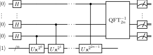
We read quantum circuits like music, left to right. Each line represents a qubit or set of qubits. Register A is shown by the lines at the top with starting state |0⟩. Register B is shown by the single line with width /n and has starting state |1⟩.
We first set register A to be all values of a < 2²ⁿ using the Hadamard gate. This is shown by the H symbols. We could have written register A with the /2n also, but we wrote register A as a series of separate lines to show that the the Hadamard gates are applied to each qubit individually.
Next we apply a series of gates to compute xᵃ mod N = k. This is shown in the circuit above as the gates marked U. Each one raising x to a different power of two controlled by a single qubit from register A. The vertical lines show the control relationship which is where the entanglement comes in.
Finally we apply the Quantum Fourier Transform to the whole of Register A and measure the results. The symbols on the right indicate that the system is measured.
How does this work quickly?
Finally Shor showed that this algorithm arrives on a prime factor of N after just a few iterations in his paper “Polynomial-Time Algorithms for Prime Factorization and Discrete Logarithms on a Quantum Computer”. Shor briefly included a proof that the algorithm above gives a prime factor of N quickly because there is at least a 50% chance of choosing a value of a that will allow us to discover a prime factor of N.
I’ll give a summary for the case where N = p₁p₂, but understanding of the proof does require a firm understanding of numerical algebra beyond the steps below. As above, start with a guess x with multiplicative order r of a mod N. Let r₁ be the order of x mod p₁ and r₂ be the order of x mod p₂. It follows, though not obviously, that r is the least common multiple (lcm) of r₁ and r₂.
xʳ¹ = 1 (mod p₁)
xʳ² = 1 (mod p₂)
Consider the largest powers of 2 that divides each of r₁ and r₂. If they are both 1 then r₁ and r₂ are odd, the lcm(r₁, r₂) is odd, so r is odd and we need to start again. It is not obvious, but if both powers of two dividing r₁ and r₂ are the same then xʳᐟ² = -1 (mod p) for both p₁ and p₂ so xʳᐟ² = -1 (mod N). This is the same as saying that N divides xʳᐟ² + 1 which we looked at above. This means that our choice of x is bad and we can’t use x to find a factor of N and we need to choose again. In our example above when x = 10, r = 6, r₁ = 6, and r₂ = 2 so both r₁ and r₂ have 2¹ as the largest power of two as a divider so our choice of x was doomed.
By the Chinese remainder theorem, picking random x < N is the same as picking random x₁ (mod p₁) and x₂ (mod p₂). This is because the theorem tells us that if p₁ and p₂ are coprime (which they are) then for any numbers x₁ (mod p₁) and x₂ (mod p₂) there is at least one number x such that x = x₁ (mod p₁) and x = x₂ (mod p₂) and that such solutions of x, x`for which that holds, x = x` (mod p₁p₂), where p₁p₂ = N. So for any x₁ (mod p₁) and x₂ (mod p₂), we could derive a unique x (mod N).
In his paper, Peter Shor shows that there is a less than 50% chance of picking x₁ and x₂ such that they share the same power of two in their prime factorisation. This means that there is a less that 50% chance of x₁ and x₂ being bad, so there is a less than 50% chance of a being bad, since choosing x₁ and x₂ is equivalent to choosing x. Therefore there is greater than 50% chance of choosing a value of x that is good.
Practicalities
There is a lot of uncertainty in Shor’s algorithm: it might take us a few goes to pick a good values of x and the continued fractions algorithm is also not guaranteed to recover our value of r. Coupled with the high error rates in quantum computers today, this means that any answers from a quantum computer need a great deal of error correction and statistical analysis to avoid additional runs of the machine. We are not yet able to build a quantum computers anywhere near the scale needed for Shor’s algorithm. It requires a large number of qubits compared with other applications of quantum computers. However with increasing investment in quantum computing it is something we should all be concerned about.